C: Granny Pie Factory 

Granny has always loved to bake pies. She has a very special recipe to prepare an apple pie. His grandson, Simon, has decided to turn Granny's hobbie into a family business. To do so, Simon has to combine two ingredients: fruit and dough. He buys these two ingredients and combines them to prepare apple pies through the appropriate process: cooking, packaging, delivering, etc.). He sells the pies to local grocery stores. As a good businessman, Simon wants to have the highest profit so he prepared a financial model for Granny Pie Factory where he defines input and output variables. Since the main idea is to get immediate profits, the only decision variable is the selling price for each pie.

As we all know, the equation to obtain the profit is as follows: Profit = Income - Costs

In order to get the cost right, Simon has to determine the process costs which he has assumed is a constant multiplied by the number of pies processed (Simon assumed that Processing Cost = 2.05*Number of pies). After several months of collecting data, Simon has realized that his assumption is false and needs to find a way to accurately predict processing costs.

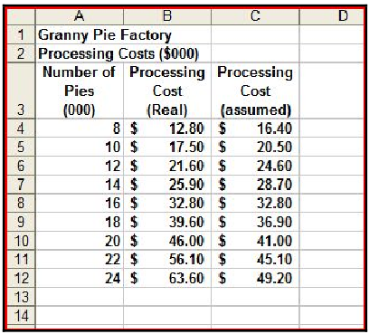
The next figure shows the data that Simon has collected

Figure 1: Granny Pie Factory Processing Cost Data

In short, the idea is to find the relationship between the number of pies processed and the processing cost.

Input 

The input consists in datasets describing the number of pies processed (in thousands), the real processing cost and the assumed processing cost. The dataset is formatted as follows.

First an integer denoting the number of pies processed followed by two reals denoting (in that order) the real processing cost and the assumed processed cost. Each number is separated by an space and there could be N lines of numbers in a dataset.

A line consisting in `0 0 0' denotes the end of the dataset.

Output 

For each dataset you will need to find the relationship between the number of pies processed and the real processing cost.

Sample Input 

8 12.80 16.40
10 17.50 20.50
12 21.60 24.60
14 25.90 28.70
16 32.80 32.80
18 39.60 36.90
20 46.00 41.00
22 56.10 45.10
24 63.60 49.20
0 0 0

Sample Output 

Linear coefficient: 0.9331
Quadratic coefficient: 0.0712

Equation: y = 0.0712 x2 + 0.9331 x